Multi-Layer Perceptrons Explained

A Beginner’s Guide to Multi-Layer Perceptrons

In this article, I will explain the intuitive workings behind Multi-Layer Perceptrons (MLPs), a critical concept in advanced neural networks. You’ll learn about the following:

1. Limitations of the Perceptron: I will explain why a single perceptron is insufficient for handling complex data.

2. The intuition behind the MLPs: You will get the essence and visualization of how the multi-layer perception works.

3. Download PDF Notes: At the end, download notes to review anytime.

What is the issue with Perceptron?

The main issue with perception is that it can only learn linearly separable patterns. It works by finding a linear boundary (decision boundary) that separates the data points of different classes. If the data is not linear, then a perception won’t be able to classify the data points correctly.

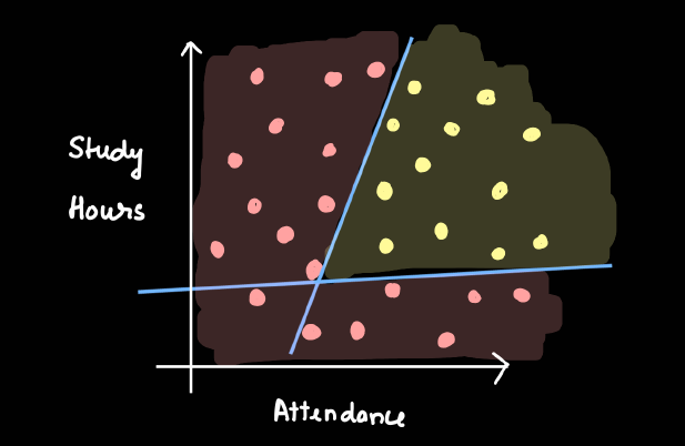
Consider a student performance dataset. We use two features, study hours and attendance, to predict whether students will pass or fail their exams. Each data point represents a student’s performance. The yellow data points indicate students who passed the exam, while the pink points represent those who failed.

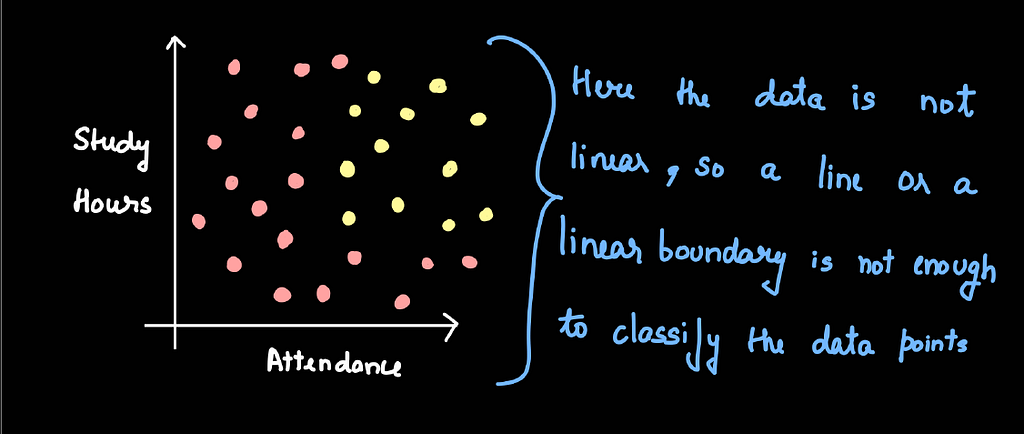
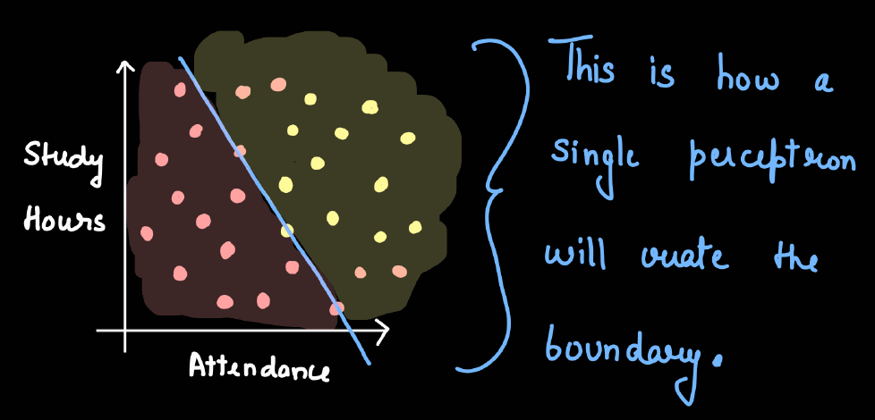
The data is not linearly separable. Therefore, a single perceptron cannot give us an ideal decision boundary that separates the data points of the two different classes. So, we can conclude that a single perceptron will work perfectly for linear data but not for non-linear datasets.

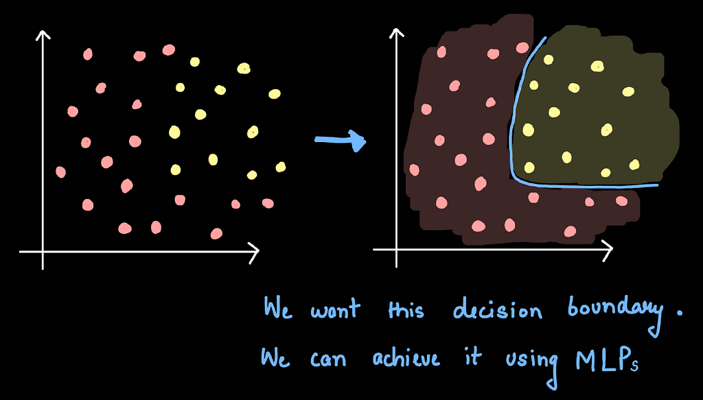
In order to correctly classify the non-linear data points, we have to use multiple perceptrons, which we will see in the next section.

The Intuition Behind Multiple Perceptrons

We have non-linear data points, as we saw in our example. Therefore, a single perceptron won’t work. Now assume that we have two perceptrons, each creating a different decision boundary, as seen in the image below. Neither of these is able to correctly classify the data points. But what if we add or superimpose the results of perceptrons 1 and 2?

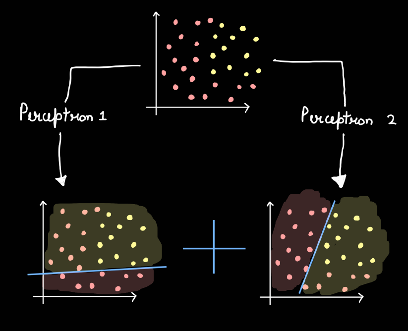
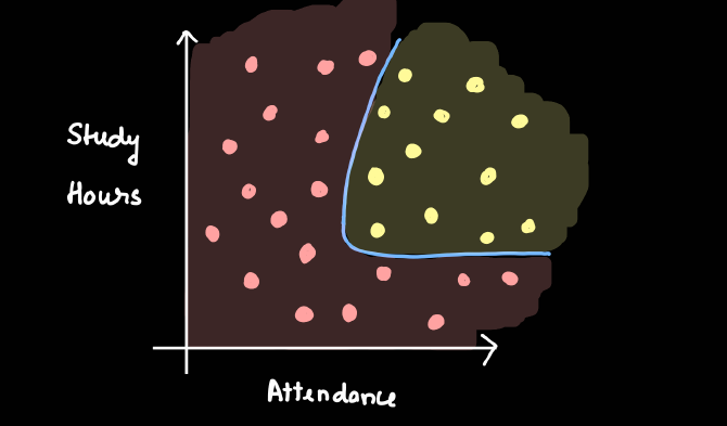
Now, let us superimpose the results of perceptron 1 and perceptron 2; the resulting graph is shown in the image below.

Now, let’s smoothen the curve, as shown in the image below. This is what we wanted from the start. Until now, I have explained it visually without delving into the mathematical details. In the next section, I will explain the mathematics behind it.

Mathematics Behind It

Let us now examine this mathematically. I randomly selected a student, as shown in the image below. The probability of this student passing the exam from perceptron 1 is 0.8, and from perceptron 2 is 0.7. The main question here is how we combine these probabilities. We cannot simply add them, as the result (0.7 + 0.8 = 1.5) would exceed 1. Therefore, after adding, we must apply the sigmoid function to bring it within the range of 0 to 1.

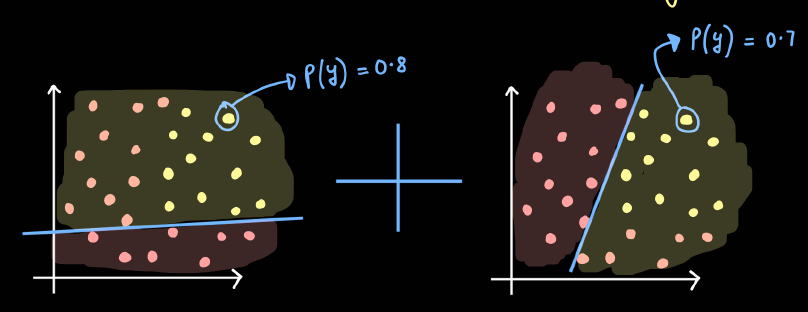
Now, add the two probabilities

Combined probability = 0.8 + 0.7 = 1.5 (Not In the range)

Apply Sigmoid function = σ(z) = σ(1.5) = 0.82

Similarly, we have to do this for every student in the dataset to get the new decision boundary.

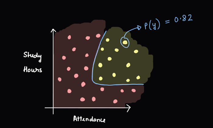
In short, we are calculating new probabilities by combining the outputs from two perceptrons. First, we add the probabilities from each perceptron. Since the sum can exceed 1, we then apply the sigmoid function to adjust these values into a valid probability range between 0 and 1. This process of adding and adjusting with the sigmoid function is crucial as it results in the superimposition and smoothing of the decision curve.

Intuition Behind Multi-Layer Perceptron

Before we move on to the multi-layer perceptron, let’s consider what factors can affect the linear combination of perceptrons. Now, I want to add more flexibility to the linear combination of multiple perceptrons by introducing the concept of weights. What if we want the output of perceptron 1 to dominate heavily compared to that of perceptron 2? As shown in the image below, the impact of the decision boundary from perceptron 1 is greater than that from perceptron 2. How can we achieve this?

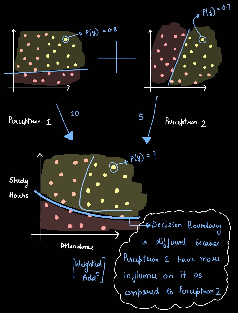
We can achieve this by performing a weighted addition of the two probabilities and assigning a specific weight to each perceptron. In our example, let’s assume the weight for perceptron 1 is 10 and for perceptron 2 is 5. After calculating the weighted sum, we apply the sigmoid function to ensure the resulting probability falls within the range of 0 to 1.

Weighted Addition : z = 10(0.8) + 5 (0.7)

Apply Sigmoid Function: σ(z)

Additionally, we can also introduce a bias to the system. Assume that the bias in the system is 3. Now, let’s perform the weighted addition again, add the bias, and then apply the sigmoid function.

Weighted Addition : z = 10(0.8) + 5 (0.7) + 3

Apply Sigmoid Function: σ(z)

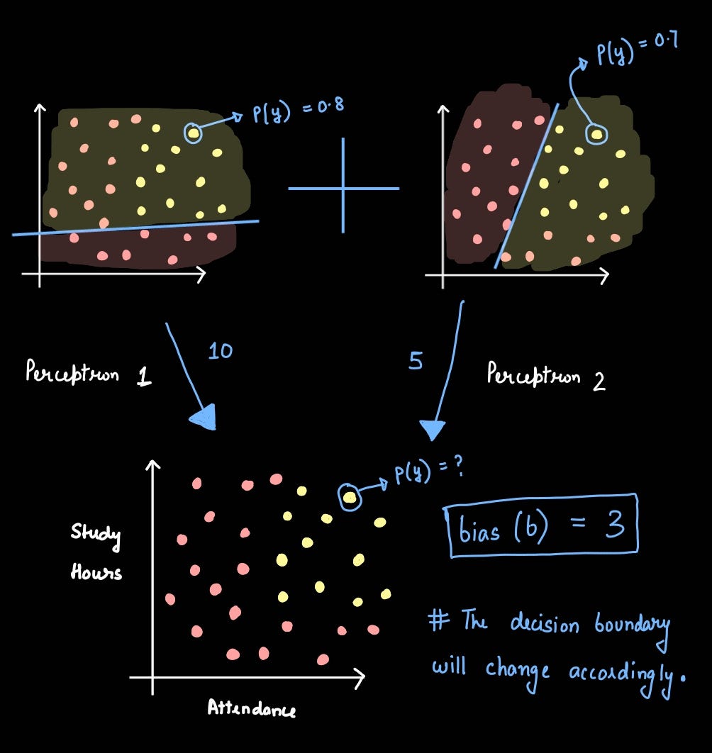
In a sense, the third white circle acts as a perceptron itself. The outputs of perceptron 1 and 2 serve as inputs for perceptron 3. Thus, we can say that we have a combination of three perceptrons, which can also be referred to as a Multi-layer Perceptron.

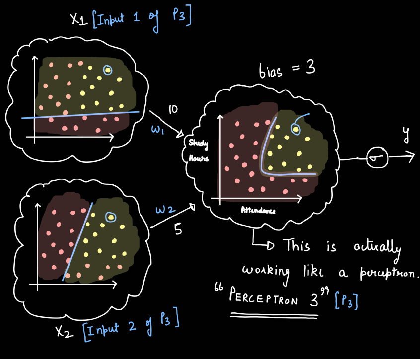
X1 is the output of perceptron 1 and W1 is the weight of the connection from perceptron 1 to perceptron 3. Similarly, X2 is the output of perceptron 2 and W2 is the weight of the connection from perceptron 1 to perceptron 2. We can also redraw the whole thing in a simple way as shown below.

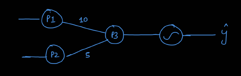
This is essentially a linear combination of perceptrons, which we refer to as a multi-layer perceptron. For a more detailed explanation, please refer to the notes provided at the end of the article.

How can we change the architecture?

The design of a basic neural network can be altered in several different ways to suit specific requirements. The approach to modifying a neural network often depends on the specific tasks we want it to perform or the particular problems we need it to solve. Below, I have outlined multiple approaches for redesigning the network’s structure.

1) Add nodes in the Hidden layer

Increasing the number of nodes in the hidden layers is akin to adding more processing power to your network. More nodes can detect more subtle and complex features in the data, which can lead to better and more nuanced predictions.

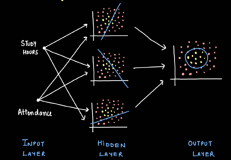
This is especially useful for complex problems where the relationships between data points are not immediately obvious.

2) Increase the number of inputs

Expanding the input layer to include more features enriches the initial data fed into the network. If we start with only two inputs, the neural network uses a simple line as a decision boundary to separate different outputs. By adding a third input, this decision boundary transforms into a plane, allowing for more complex and nuanced separations between categories.

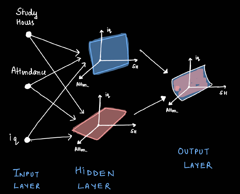
As we continue to add more inputs, these decision boundaries evolve into multi-dimensional shapes. This enhancement significantly improves the network’s ability to classify data accurately.

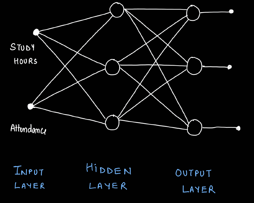
3) Add nodes in the Output layer

When we add nodes to the output layer of a neural network, it allows the network to make more distinctions among the outputs it produces. Initially, if the network is designed to make simple decisions, like categorizing images as either cats or dogs, it may only need two output nodes — one for each category. However, if we want the network to differentiate between various breeds within those categories, adding more nodes to the output layer becomes necessary.

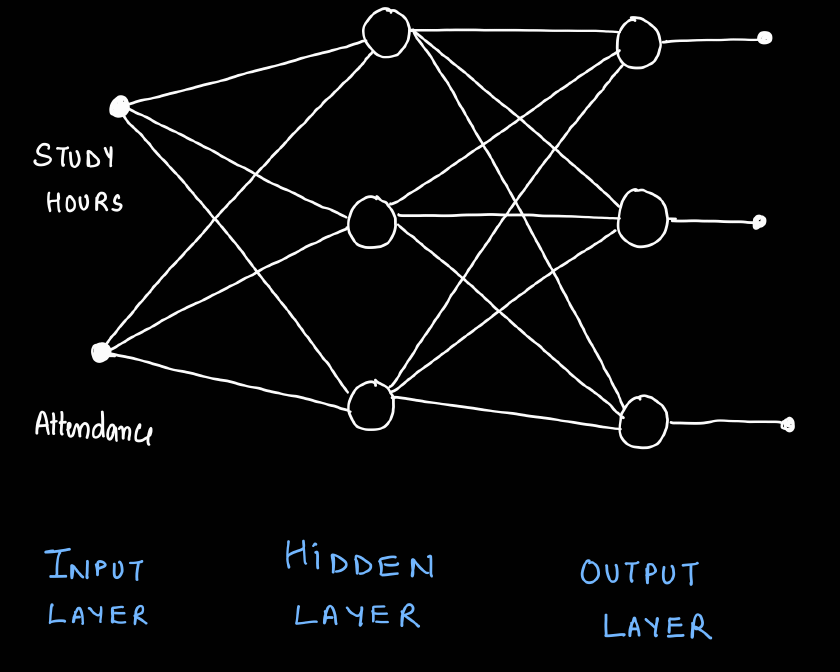
For example, suppose we want our network not just to recognize cats and dogs, but to identify specific breeds like Siamese, Persian, Labrador, and Golden Retriever. In this case, we would add more nodes — each one corresponding to one of these breeds. This way, each additional node can represent a new category, which allows the network to classify inputs into more specific groups.

4) Add more hidden layers

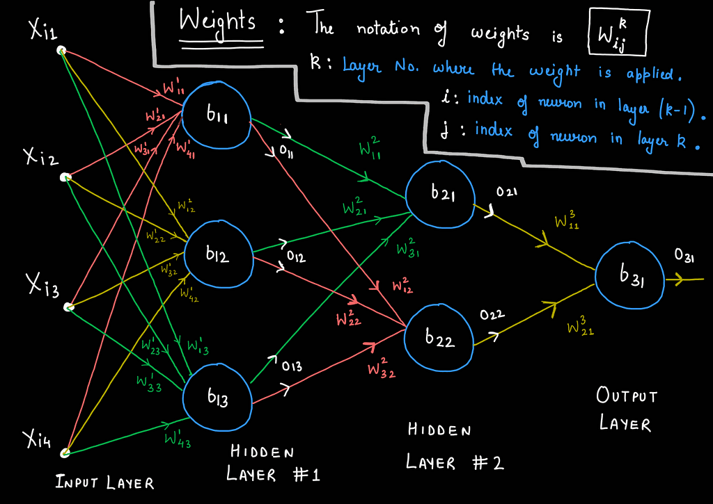
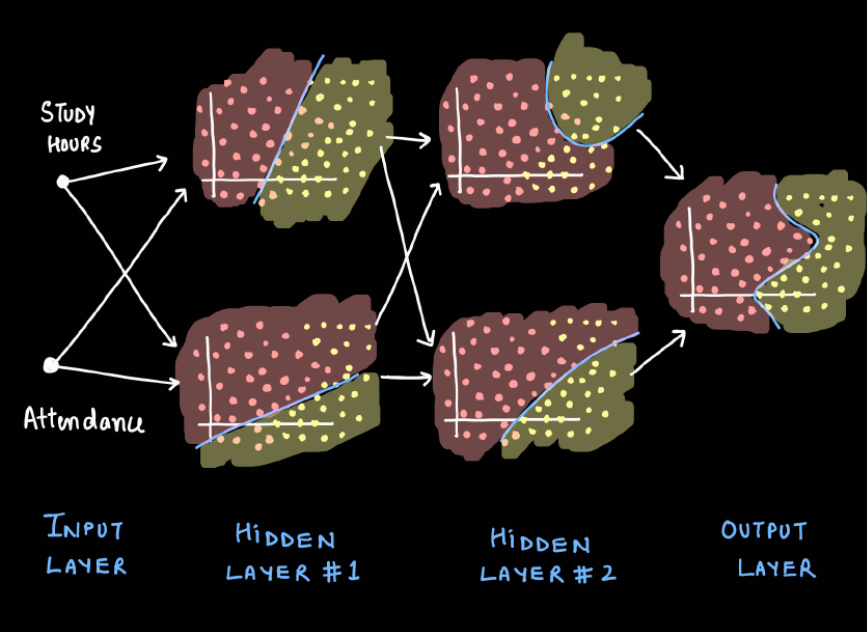
Adding more hidden layers to a neural network, as illustrated in the image below, is like adding extra levels of processing or filtering to enhance its understanding of the input data. With a single hidden layer, the network might only be able to make basic predictions based on direct relationships, such as more hours studied leads to better performance. However, by adding a second hidden layer, the network can start to understand more complex patterns, such as how consistent study habits over time, combined with regular attendance, might influence performance differently than just cramming before exams.

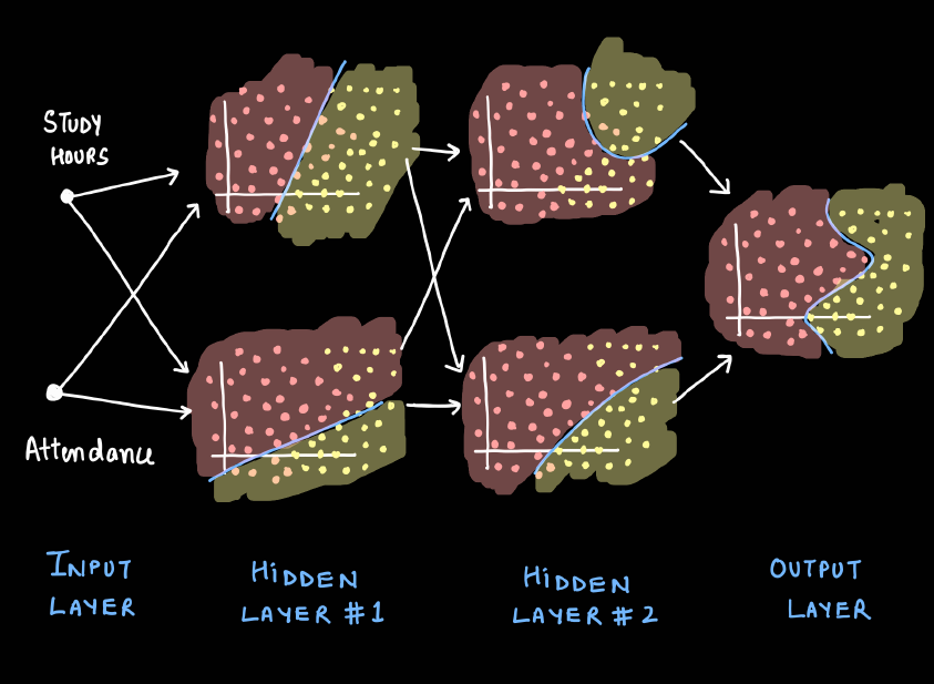
Each layer in a multilayer network can learn different aspects of the data. The first hidden layer might detect simple patterns, while the second layer builds on those findings to recognize more abstract concepts. This layering effect enables the network to make more nuanced decisions based on deeper insights into the data.

Adding more hidden layers can significantly increase the learning capability of the network, allowing it to solve more complex problems. However, it’s important to balance the number of layers with the available data and computational resources, as too many layers can lead to overfitting, where the model learns the training data too well but performs poorly on new, unseen data.

Download the PDF Notes

To make your learning easier, I’ve compiled all the key concepts, diagrams, and explanations from this article into a downloadable PDF file. This resource will serve as a quick reference guide for understanding the multi-layer perception.

👉 [Click here to download the PDF notes]

Keep this resource handy while working on your MLP projects or revising key concepts.

Don’t forget to follow me for more such content! 🚀